Science Data Pipelines
The main task of the Science Data Pipelines (SDP) is to process all WFI spectroscopic data, produce Level-4 grism and prism science data products, and deliver these data products, along with information on data quality, to the Roman archive.
Science Data Pipelines (SDP)
The SDP is made up of two parts. The first part, the G2DP, is designed to calibrate the 2D grism and prism science data and produce 1D spectra for each identified source. The second part, the G1DP, is designed to analyze and extract basic information from the 1D spectra, namely, redshifts and emission/absorption line parameters, for each target. The requirements to produce the 2D and 1D spectra, and the basic measured parameters, are common to both the grism and prism data.
The algorithms for data reduction and spectral fitting are based on those used in the Euclid SIR (Spectroscopy-IR; 2D spectroscopy processing element) and SPE (Spectroscopy; 1D Processing Element) functions. The basic functions of the G2DP and G1DP are shown in Figure 2 and described briefly, below.
The basic steps of the SDP are:
- Identification and position measurement of all spectra
- Spectral flat fielding
- Background identification and subtraction
- Identification and removal of contaminating sources, producing decontaminated 2D spectral cutouts
- Extraction of 1D spectra from the 2D cutouts
- Relative and absolute flux calibration of the 1D spectra
- Combination of 1D spectra from different exposures, dithers, and/or rolls
- Fitting of the 1D spectra to produce redshifts and other spectral feature parameters.
Level-3 and Level-4 image data products are inputs to the SDP and are used in conjunction with the Level-2 spectroscopic data to identify and extract sources from the grism and prism data. Calibration reference files produced in the Calibration Data Pipeline (CDP) are used as inputs to the SDP to calibrate the grism and prism science data.
Roman slitless spectroscopic data will suffer from cross-contamination from sources located close enough in the sky that their spectral footprints overlap. A typical galaxy will be dispersed by the grism across 90 arcseconds of sky and cover an area of more than 5000 pixels. With expected spectroscopic source densities approaching ~105 deg-2 (at H < 22.5 AB mag), overlapping spectra will be common. To illustrate this, a simulated H- band image and corresponding set of grism spectra across ½ of one WFI chip is shown in Figure 3. Spectral images for the prism will be much shorter, but overlap of spectra will still occur and have to be tracked during pipeline data processing

Figure 2: Basic data flow through the GDPS 2D (G2DP) and 1D (G1DP) components of the Science Data Pipeline (SDP). Imaging and basic spectroscopic data products from the Science Operation Center (SOC) enter the G2DP at the top left. Rough divisions between Level-2 and Level-4 Roman data levels for the grism and prism data are indicated on the left. Calibration reference files, derived in the Calibration Data Pipeline (CDP) from dedicated calibration observations, are used in the SDP and enter at the upper right. The 1D extracted spectra from the G2DP are the primary inputs to the G1DP. Additional reference files (e.g., spectral templates, line lists, grism and prism parameter files, etc.) that are inputs for the G1DP are indicated on the right.

Figure 3: Simulations (direct H-band (left), grism (middle), prism (right)) based on Wang et al. (2022) mock catalogs. All three panels are of same simulated area of sky, ~28 arcmin2 taken from SCA 1. The simulated exposure time is 300 seconds for the grism. Rough wavelengths for the bottom/top of each dispersed spectrum are indicated to the right of the grism/prism images. There are ~2000 galaxies down to H~25 mag in the direct image. The image contains about 500 objects with H < 22.5 mag AB, roughly the dividing line for significant grism continuum detection in a single 300 sec image. For comparison, we expect roughly 100 line emitters with line flux > 1×10-16 ergs cm-2 s-1 in the same region.
GDPS 2D Pipeline (G2DP)
Individual pipeline modules in the G2DP include:
- WCSUpdate: Measure blue edge positions for bright point sources to update positions of spectra
- CoordMapping: Convert RA+Dec catalog into bounding boxes for dispersed images
- 2DStamps: Cut out small stamp images from direct image for input sources
- FlatField: Apply small-scale flat field (based on background zodiacal light) to input grism/prism
- Bkgd_Large: Fit and subtract large-scale diffuse background component
- ContamIdentify: For each 2D spectrum, identify all contaminating sources
- Decontamination: Model contaminating spectra and subtract them from each source
- 1DExtract: Extract 1D spectrum from each 2D spectrum, applying wavelength solution
- FluxCal_Relative: Apply relative flux calibration cube to 1D spectra to correct for large-scale illumination pattern
- FluxCal_Absolute: Apply absolute flux calibration to 1D spectra to produce flux-calibrated 1D spectra.
- SpectraCoadd: Weighted co-addition of spectra from all available dithers/rolls.
These modules take as input the Wide-Field Spectroscopy Mode (WSM) images and catalogs, WSM spectra, and the calibration reference files from the CDP.
The ContamIdentify and Decontamination modules are particularly critical steps of the pipeline, and these are outlined diagrammatically in Figure 4.

Figure 4: Spectral and imaging data are used to remove contaminating, overlapping spectra for each science target. Output is a clean, 2D spectrum for each detected source.
Recommendations for Wide Field Spectroscopy Mode Supporting Images:
Level 3 images, and a derived Level 4 catalogs of the same region of the sky are required to run the G2DP pipeline and process any Level 2 grism or prism data. Therefore all spectroscopy, grism or prism, requires direct imaging in at least one filter in order for the source spectra to be extracted by the pipeline. While the spectroscopy pipeline will operate with only a single band of direct imaging, it is recommended that at least two filters are used, as the decontamination algorithm (see above) regularly builds model SEDs based on the measured direct imaging photometry alone. With only a single filter, the decontamination algorithm has no information on the source color and will fit unreliable SED models and consequently produce unreliable decontamination. The more direct filters that sample the wavelengths covered by the grism (1-1.93 μm) or prism (0.75-1.8 μm), the more reliable the photometry SED models will be. The expectation is that three filters should be sufficient for most decontamination modeling.
Roman WFI direct imaging is much more sensitive than WFI spectroscopy, achieving a 5σ direct image detection of a source 150x faster than a comparable continuum resolution element for the more sensitive prism. The speed difference for the grism is in the thousands. For most observations, the length of the required accompanying direct imaging should therefore be driven by the needs for producing quality direct imaging (dithering, overhead-to-science time efficiency, other science goals, etc.) rather than trying to match the spectroscopy depths. However, as a general guideline for best spectroscopy extraction, one should determine the continuum depth in spectroscopy they wish to achieve and then make sure the accompanying direct imaging is sensitive enough to detect that source at a minimum 10σ, or preferably greater than 20σ. The higher S/N in the direct images produces more accurate source positions and consequently more accurate wavelength and redshift solutions.
GDPS 1D Pipeline (G1DP)
The G1DP involves two primary steps -- redshift measurement and spectral feature measurement. The redshift measurement is based on a noise-weighted, least-squares fitting of a model to the extracted and calibrated 1D spectra. In addition to redshift, the pipeline returns the best-fit model parameters: spectral template, line ratio template, interstellar absorption on the continuum and emission lines (independently) and intergalactic absorption. Errors in the fitting are propagated in all procedures and used to derive an estimate of the error in the measured line characteristics. Estimation of higher order astrophysical parameters (e.g., extinction, star formation rate, star formation history) will be done by science teams. The spectral feature measurement is where lines are fit (both with a gaussian and direct integration) using the redshift and classification returned by the redshift measurement. An assessment of the reliability of the redshift measurement is performed by an additional step, the Redshift Reliability module. The steps in G1DP are outlined diagrammatically in Figure 5.
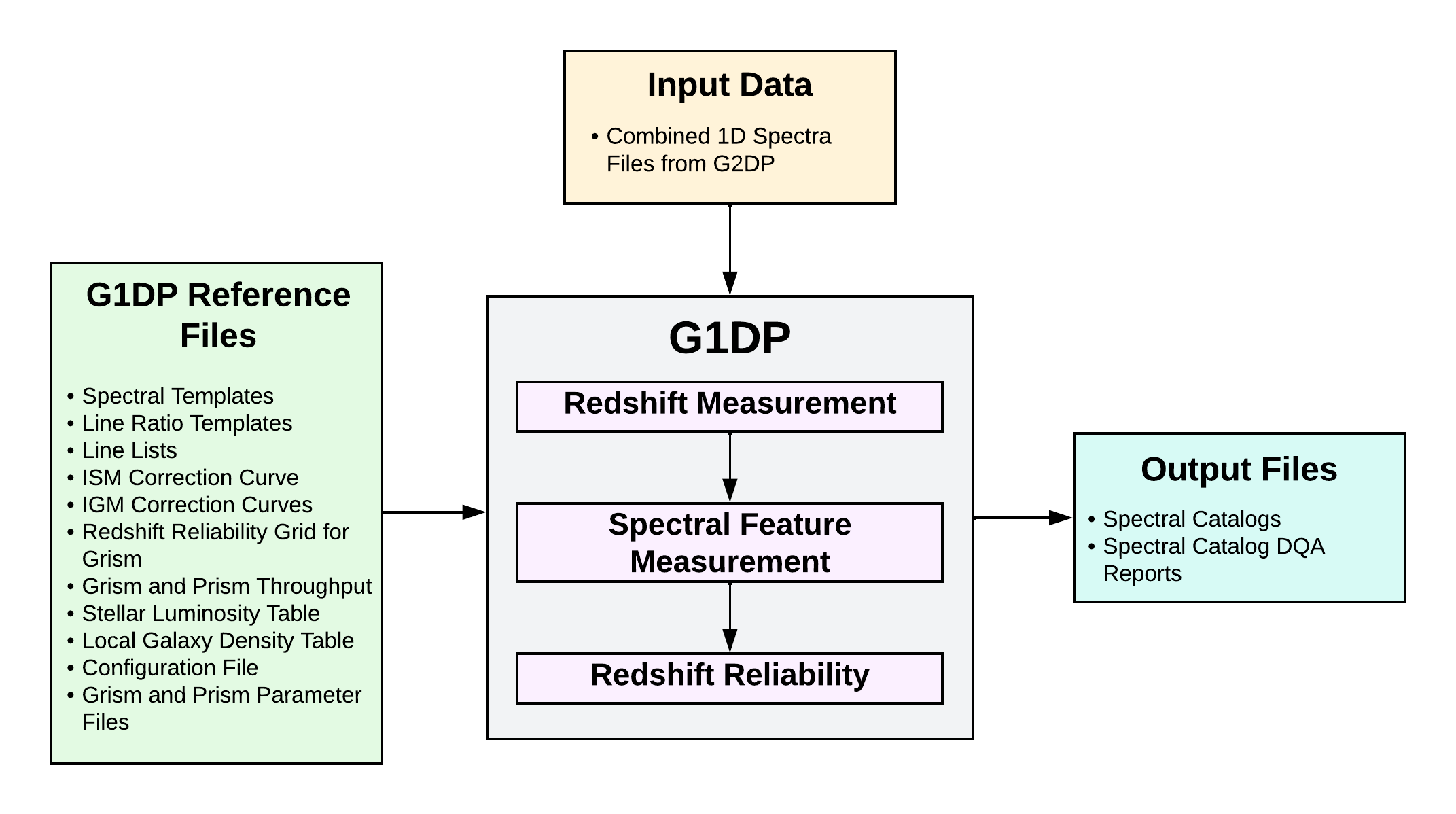
Figure 5: The G1DP consists of three primary components: Redshift Measurement, Spectral Feature Measurement and Redshift Reliability. The input data are the Combined 1D Spectra files from G2DP that contain the flux-calibrated 1D spectra with uncertainties and line-spread functions (among other results). All the G1DP Reference Files are listed in the figure above and are required for G1DP processing. The outputs are the Spectral Catalogs and the Spectral Catalog DQA Reports. The catalogs include results such as: the best redshift measurement with uncertainty, the redshift probability distribution function (zPDF), the best-fit spectral template, redshift reliability estimation, and detailed spectral line properties (e.g., wavelength, flux, equivalent width, velocity).
G1DP Overview:
The G1DP contains three related modules: Redshift Measurement, Spectral Feature Measurement and Redshift Reliability.
The primary spectral input data are the Combined 1D Spectra files that have been created in G2DP. Specifially, G1DP uses the 1D spectra (wavelength, flux and flux error), line spread functions, and peak signal-to-noise measurement of the spectrum from these files (along with some other metadata information). The G1DP will run on objects returned by G2DP that meet basic signal-to-noise and brightness requirements. To include families of "line-only" sources, a peak signal-to-noise measurement is used for the signal-to-noise cut, which uses a moving window filter to measure excess signal over a specific wavelength region.
The grism and prism parameter files contain the detailed choices made for each module and each object type (e.g., redshift range, redshift step, redshift fitting method). The two primary modules (Redshift Measurement and Spectral Feature Measurement) are executed for the classified object type (galaxy, quasar, star, and supernova). Note, that the supernova object type is only available when fitting Roman prism spectra. The third module, Redshift Reliability, is only executed for grism observations where the spectrum is classified as a galaxy.
The G1DP creates two types of files: a spectral catalog (parquet format) and spectral catalog DQA report (pdf). There is a separate catalog for each optical element (grism or prism) and observational program. Within the catalog, each spectrum has its own row which contains all the results of G1DP corresponding to that spectrum. A single catalog may be spread across several files just to keep the file size manageable. A separate spectral catalog DQA report file is created for each catalog file. Catalogs will be created periodically (roughly every three months) and final catalogs will be created at the end of each observational program.
The G1DP creates intermediate spectral files, which are not currently saved. These intermediate files include a single output parquet file that contains results from all the spectra contained in a single field-of-view.
Figure 6 describes the processing of an individual Roman 1D spectrum in more detail.

Figure 6: Diagram of the G1DP processing for a single spectrum. The redshift measurement step of the G1DP is shown in detail. The redshift is fit independently for every object type. Then the Redshift Measurement classifies the spectrum as the object type that had the best fit. After determining the best fit redshift and object type, the Spectral Feature Measurement module is evaluated using the best fit redshift result for the classified object type. Finally, the Redshift Reliability module returns the reliability index for grism observations if the object is classified as a galaxy.
Redshift Measurement:
The Redshift Measurement module measures the best fit redshift assuming that the spectral object is a galaxy, quasar, star, and supernova (for the prism). All fits are performed using noise-weighted least-squares fitting. The Redshift Measurement module also determines what object class best matches the input 1D spectrum.
Each class, or object type, has a set of unique parameter files, including a set of spectral templates and a line catalog. The estimate of the redshift for each 1D spectrum is calculated in two “passes”. First, the module finds the best fit for each redshift in a coarse redshift grid (Δz = 10-3 for the galaxy fit). To find the best fit at the given redshift, the module uses a redshift fitting method (see below for a description of the two different methods used) to fit the optimum model (i.e. set of scaled templates/catalogs) to the observation and then determines the ꭓ2 = Σλ(fobs - fmodel)2/(σobs)2 of that fit, where f is the flux and σ is the flux error at a given lambda. The second pass is a fine grid (Δz = 10-4 for the galaxy fit) centered on the best redshifts found in the first pass. In the second pass, the module also smooths the spectral template to match the observed line spread function and corrects for interstellar and intergalactic absorption features, if appropriate. The model (used in the redshift measurement) includes a fit of the Lyman-alpha line profile, independent of the other emission lines.
The ꭓ2 at each redshift in the second pass is converted into the redshift probability distribution function (zPDF). The best fit redshift is given by the position of the highest peak of the zPDF. Secondary peaks (up to 2) in the zPDF indicate other, less likely, but possible redshift solutions. The redshift error is the FWHM of a gaussian fitted to the zPDF at the candidate’s redshift. The probability that the candidate redshift is correct is the fractional area under a gaussian fitted to the zPDF at that redshift, to the total integrated zPDF.
Once the best redshift is found for each object type, a Bayesian model selection classifies the final object type. The likelihood (at all z) for each type is integrated over the whole z range (or velocity for stars). The type with highest evidence is then chosen. The code computes the posterior probability of being a galaxy, quasar, star, or supernova, assuming equiprobability, a priori.
The SED fit parameters should be considered preliminary values, useful for planning further analysis, since these parameters are returned from the fitting procedure, whose primary goal is to determine the redshift. Further estimates of higher-order astrophysical parameters (e.g., extinction, star formation rate, star formation history, etc.) will require more detailed fitting by the science teams. Specifically for the prism data, host galaxy subtraction and SN typing are assumed to ultimately be the responsibility of the Roman science teams.
There are two different redshift fitting methods employed by the G1DP.
The first method (by default only used for galaxy fits) is called LineModelSolve. First the method scales a spectral template (at the redshift currently being evaluated) to subtract the continuum from the spectrum. During this process the method masks out all the lines that appear in the line catalog, so only the continuum is fitted and subtracted. Next, the method scales the line ratios in the line catalog to match the continuum-subtracted observation. During this line catalog fit, there are two velocity dispersion parameters calculated: one for all emission lines and one for all absorption lines. The scaled spectral template and line catalog are added to create a model spectrum. The fit of this model to the observed spectrum is evaluated by the ꭓ2. After doing this for every combination of spectral template and line catalog, the method selects the model (combination of spectral template and line catalog) with the smallest ꭓ2. That ꭓ2 value is returned as the metric of how well that object type fits the observation at the given redshift.
The second method (by default used for the quasar, star and supernova fits) is called TemplateFittingSolve. The method simply scales a spectral template (at the redshift currently being evaluated) and calculates the ꭓ2 for this fit. With this redshift fitting method, the model is simply the scaled spectral template. After doing this for every spectral template, the method selects the model with the smallest ꭓ2 value.
Spectral Feature Measurement:
The inputs to the spectral feature measurement module are (1) a line catalog for the classified object type and (2) the best fit redshift from the Redshift Measurement module. The best fit redshift is assumed to be correct and is used to redshift the line catalog to match the observed spectrum. For each emission and absorption feature in the line catalog, a local estimate of the continuum is done by fitting a quadratic function to the emission on either side of the line (given the input LSF). This continuum fit is then subtracted to measure the properties of the emission or absorption feature (e.g., line flux and equivalent width). Errors in the fitting are propagated in all procedures and used to derive an estimate of the error in the measured line characteristics.
Redshift Reliability:
The zodiacal background, local stellar density and local galaxy density are calculated by this module for every spectrum. However, the redshift reliability index is only calculated for grism observations when the spectrum is classified as a galaxy. The input files used to estimate the redshift reliability are the data and corresponding grism reliability “grid”. This grid allows for a rough, quantitative assessment of the reliability of a particular galaxy redshift, by matching the details of its associated observation with the grid of observational parameters. The final grid will be created during the early stages of the Roman mission. Each galaxy spectrum is assigned a Redshift Reliability index based on seven grid parameters: (1) the measured redshift found in the Redshift Measurement module, (2) the maximum signal-to-noise ratio of a line found in the Spectral Features Measurement, (3) the number of exposures in the observations, (4) number of roll angles in the observations, (5) the zodiacal background, (6) the local stellar density and (7) the local galaxy density. Multiple, repeated observations of the same field will be used to create the final reliability grid. The Redshift Reliability index ranges from 1 to 4 with 1 being the most reliable and 4 being the least reliable.
Archived Products:
- Spectral Catalog
- Parquet format
- Contents include:
- List of best redshifts
- Redshift errors
- zPDF
- Best fit template based classification
- Line wavelengths
- Line fluxes
- Equivalent widths
- Redshift reliability index
- Spectral Catalog DQA (Data Quality Assessment) Report
- Contents include:
- Global statistics
- Number of each classified object type
- Fraction of objects with redshifts and radial velocities measured
- Plots
- Histogram of the redshifts measured (separated by object type)
- Histogram of the radial velocity measured for stars
- Histogram of the maximum line signal-to-noise per spectrum
- Global statistics